In sectors such as energy, water, or transportation, detecting an operational failure minutes—or days—before it occurs can mean the difference between a planned intervention and a production breakdown. This explains how anomaly detection models work in time series and what technical criteria guide their selection.
What is an anomaly in a time series?
An anomaly in time series is any observation that deviates significantly from the expected behavior given the historical context, trend, and seasonality of the data. The difficulty lies not in defining it, but in identifying it automatically and robustly in continuous data streams.
It is necessary to distinguish between three main types, and understanding which type the phenomenon we want to detect belongs to directly influences the model architecture:
- Point Anomaly
An individual value deviates extremely from the usual range. Example: a peak in electricity consumption 10 times the average at a specific moment. These are the easiest to detect but also the most prone to false positives if the model doesn’t consider the temporal context.
- Collective Anomaly
A sequence of points that, taken individually, seem plausible, but whose combined pattern is anomalous. The classic example in utilities is a sustained drop in flow rate over several hours with no recorded operational cause—each individual reading falls within range, but the aggregate trend reveals a progressive loss.
- Interval Anomaly
A time window where the behavior deviates from the expected seasonal pattern. This is especially relevant in transportation: unusually low occupancy during peak hours can indicate a service problem that point-oriented models would never detect.
Challenges Inherent to Operational Data
Critical sectors (energy, transportation, etc.) introduce challenges that don’t appear in laboratory datasets:
Multi-level seasonality
A power grid sensor has simultaneous daily, weekly, and annual periodicity. A model that doesn’t properly decompose these anomalies will generate thousands of false alarms.
Missing and corrupted data
Field sensors fail, and SCADA protocols have latencies. An anomaly model that doesn’t distinguish between “missing data” and “actual anomalies” is useless in production.
Concept drift
The “normal” behavior of a network changes when infrastructure is expanded, consumption patterns change, or operations are reconfigured, in this case, the model must be updated.
High cost/benefit asymmetry
A false negative (undetected anomaly) in a pressurized water pipe has very different consequences than a false positive. Calibrating the alert threshold is as critical as the model itself.
Models: from classical statistics to deep learning
The decision of which model to apply should be based on the characteristics of the data and the operational cost of each type of error, not on the most fashionable algorithm. Here is an honest map of the ecosystem:
| Model | Paradigm | Best for | Main limitation | Required data |
|---|---|---|---|---|
| ARIMA / SARIMA | Statistical | Stationary time series with known seasonality | Requires stationarity; performs poorly with non-linearities | Low |
| Holt-Winters | Exponential smoothing | Forecasting with double seasonality | Assumes fixed seasonal structure | Low |
| Prophet | Bayesian additive | Time series with calendar effects, holidays, and trends | Less accurate at high frequency (seconds-level data) | Medium |
| LSTM / GRU | Recurrent deep learning | Complex temporal patterns, multivariate series | Requires large datasets; black-box model | High |
Application in sectors and businesses: what anomalies to detect in each context
Below are some examples of use cases in different sectors, where the anomaly taxonomy and model selection become meaningful when applied to real operational scenarios, the most commons in each sector are:
- Energy
Transformer degradation detected by collective anomalies in temperature and load. Detection of unjustified technical losses in network segments. Uncorrelated increase between generation and billed energy.
- Water and Utilities
Leaks detected through nighttime flow analysis. Contamination due to anomalies in conductivity and turbidity sensors. Detection of anomalous consumption indicating unreported leaks.
- Transportation and Mobility
Asset degradation (tracks, motors) due to vibration and temperature. Irregularities in the headway that anticipate saturations. Anomalous occupancy at nodes indicating upstream service failures.
In all cases, the value lies not only in detecting the anomaly, but also in the ability to anticipate it. A model that identifies transformer degradation 72 hours in advance allows for intervention planning. If detection occurs only minutes before the failure, its usefulness is limited to subsequent analysis.
Production Pipeline: Beyond the Model
The most frequent mistake in anomaly detection projects is treating the model as the final product. In operational environments, the model is a component of a pipeline that needs to be fully designed from day one:
1) Ingestion and Preprocessing
Unification of heterogeneous sources (SCADA, IoT, ERP), normalization, gap interpolation. Data quality is the most common bottleneck in production.
2) Temporal Feature Engineering
Construction of lag features, rolling statistics, and seasonal decomposition. Good feature engineering is often more valuable than a more complex model.
3) Training and Validation
Walk-forward validation (no random train/test split: temporal data is time-dependent). Threshold selection using curves such as Precision-Recall.
4) Alert Deployment
Integration of the anomaly signal into existing operational workflows: maintenance tickets, control dashboards, and on-call notifications. Without this integration, the model has no impact.
5) Monitoring and Retraining
Monitoring data drift and model drift. Periodic or triggered retraining; without this loop, models silently degrade.
How LUCA BDS 4.0 Addresses These Challenges
With this new actualitation of LUCA BDS, the platform reinforces its position as a key layer for bringing advanced analytics, including time-series anomaly detection, from the lab to real-world operations.
LUCA BDS incorporates capabilities that allow organizations in sectors such as energy, water, and transportation to:
- Unify and leverage time-series data at scale: native integration of heterogeneous sources (IoT, SCADA, enterprise systems), facilitating a consolidated and contextualized view of operational behavior.
- Activate anomaly detection use cases: by combining advanced analytics, business rules, and the integration of external models, enabling the identification of relevant deviations in critical metrics.
- Operationalize analytics: transforming analytical signals into actionable alerts, integrated into dashboards and decision flows, reducing time-to-action.
- Integrate with the data science ecosystem: the ability to consume results from models developed in environments like Python or Spark, seamlessly incorporating them into the analytics layer.
- Deploy in secure and controlled environments: on-premises or private execution, guaranteeing data sovereignty and regulatory compliance.
In this approach, LUCA BDS doesn’t compete with machine learning frameworks, but rather enhances them: it acts as the platform that allows anomaly detection models to scale, industrialize, and be implemented commercially, closing the complete cycle between data, analysis, and decision.
Webinar: Machine Learning applied to the early detection of anomalies
Led by Marcos Cobo (Head of AI and Data), this webinar explains how LUCA BDS helps detect anomalous behavior, anticipate deviations, and generate early warnings in time-series data to improve efficiency and service continuity.
The session content is structured around the following key areas:
- Introduction to the LUCA BDS 4.0 AI engine.
- How to apply AI and machine learning to time series data.
- Live demonstration of LUCA BDS.

Want to see these AI techniques in action on real data?
Fill out the form to download the webinar